[Image1]
Introduction
Hey it's a me again @drifter1!
Today we continue with my mathematics series about Signals and Systems in order to cover Processing Continuous-Time Signals as Discrete-Time Signals.
So, without further ado, let's get straight into it!
Continuous-Time to Discrete-Time Conversion (and vise versa)
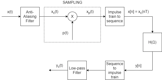
Maybe the most important application of sampling is its role in processing continuous-time signals using discrete-time systems. Continuous-Time signals have to be band-limited in order for the conversion to work. If they are already band-limited they can easily be sampled, and those samples are then converted to some kind of discrete-time representation. On the other hand, if they are not band-limited that are first processed with an anti-aliasing filter (which band-limits them) and then sampled.

The resulting discrete-time representation of the continuous-time signals can be processed by discrete-time systems and when the whole procedure is finished desampled/reconstructed into continuous-time signals. This is done using preferably band-limited interpolation, which allows converting the sequence to an (im)pulse train. This (im)pulse train is then processed through a low-pass filter, which in turn gives the final continuous-time signal. Of course the exact sampling period, the periodicy of the to-be-sampled signal, and much much more that we already discussed throughout the series, also affects the outcome of this whole procedure.
Discrete-Time Processing
Whilst converting the impulse train of samples to a sequence of samples, we basically normalize the time-axis. Recalling the properties of the Fourier Transform, its easy to conclude that the discrete-time Fourier transform of the sequence of samples gives the same result as the continuous-time Fourier transform of the impulse train, if the frequency-axis is normalized in that case. In other words, processing the continuous-time signal as an discrete-time signal is not violating the Fourier transform principles, and the result after the sampler is the same that we would get processing the continuous-time signal directly.
To get even more specific, while converting the result back to a continuous-time signal, we basically "un-normalize" the frequency-axis. So, the overall system which processes the discrete-time representation is equivalent to a continuous-time filter with a frequency response that is the same as the frequency resposne of the discrete-tiem filter if linear scaled on the frequency-axis. The cut-off frequency in this case depends on the sampling frequency, and so it can be varied by varying the sampling frequency.
Complete Block Diagram

RESOURCES:
References
Images
Mathematical equations used in this article were made using quicklatex.
Block diagrams and other visualizations were made using draw.io and GeoGebra
Previous articles of the series
Basics
- Introduction → Signals, Systems
- Signal Basics → Signal Categorization, Basic Signal Types
- Signal Operations with Examples → Amplitude and Time Operations, Examples
- System Classification with Examples → System Classifications and Properties, Examples
- Sinusoidal and Complex Exponential Signals → Sinusoidal and Exponential Signals in Continuous and Discrete Time
LTI Systems and Convolution
- LTI System Response and Convolution → Linear System Interconnection (Cascade, Parallel, Feedback), Delayed Impulses, Convolution Sum and Integral
- LTI Convolution Properties → Commutative, Associative and Distributive Properties of LTI Convolution
- System Representation in Discrete-Time using Difference Equations → Linear Constant-Coefficient Difference Equations, Block Diagram Representation (Direct Form I and II)
- System Representation in Continuous-Time using Differential Equations → Linear Constant-Coefficient Differential Equations, Block Diagram Representation (Direct Form I and II)
- Exercises on LTI System Properties → Superposition, Impulse Response and System Classification Examples
- Exercise on Convolution → Discrete-Time Convolution Example with the help of visualizations
- Exercises on System Representation using Difference Equations → Simple Block Diagram to LCCDE Example, Direct Form I, II and LCCDE Example
- Exercises on System Representation using Differential Equations → Equation to Block Diagram Example, Direct Form I to Equation Example
Fourier Series and Transform
- Continuous-Time Periodic Signals & Fourier Series → Input Decomposition, Fourier Series, Analysis and Synthesis
- Continuous-Time Aperiodic Signals & Fourier Transform → Aperiodic Signals, Envelope Representation, Fourier and Inverse Fourier Transforms, Fourier Transform for Periodic Signals
- Continuous-Time Fourier Transform Properties → Linearity, Time-Shifting (Translation), Conjugate Symmetry, Time and Frequency Scaling, Duality, Differentiation and Integration, Parseval's Relation, Convolution and Multiplication Properties
- Discrete-Time Fourier Series & Transform → Getting into Discrete-Time, Fourier Series and Transform, Synthesis and Analysis Equations
- Discrete-Time Fourier Transform Properties → Differences with Continuous-Time, Periodicity, Linearity, Time and Frequency Shifting, Conjugate Summetry, Differencing and Accumulation, Time Reversal and Expansion, Differentation in Frequency, Convolution and Multiplication, Dualities
- Exercises on Continuous-Time Fourier Series → Fourier Series Coefficients Calculation from Signal Equation, Signal Graph
- Exercises on Continuous-Time Fourier Transform → Fourier Transform from Signal Graph and Equation, Output of LTI System
- Exercises on Discrete-Time Fourier Series and Transform → Fourier Series Coefficient, Fourier Transform Calculation and LTI System Output
Filtering, Sampling, Modulation, Interpolation
- Filtering → Convolution Property, Ideal Filters, Series R-C Circuit and Moving Average Filter Approximations
- Continuous-Time Modulation → Getting into Modulation, AM and FM, Demodulation
- Discrete-Time Modulation → Applications, Carriers, Modulation/Demodulation, Time-Division Multiplexing
- Sampling → Sampling Theorem, Sampling, Reconstruction and Aliasing
- Interpolation → Reconstruction Procedure, Interpolation (Band-limited, Zero-order hold, First-order hold)
Final words | Next up
And this is actually it for today's post!
Next time we will get into discrete-time sampling...
See Ya!

Keep on drifting!
