[Image1]
Introduction
Hey it's a me again @drifter1!
Today we continue with my mathematics series about Signals and Systems in order to cover Filtering.
So, without further ado, let's dive straight into it!
Convolution Property
Before we get into Filtering, its wise to recall the convolution property of the Fourier transforms, as this property is the foundation Filtering is built upon.
In either Time-Domain, the convolution of two signals turns into multiplication in their Fourier Transforms:

In the exercises about LTI systems, this property helped us simplify the calculations for the system response/output. Moving into the Frequency-Domain turned all the complicated convolution calculations into simple multiplications of known Fourier Transforms. To get even more specific, in LTI systems the Fourier transform of the output is equal to the Fourier transform of the input multiplied by the frequency response, which in turn is simply the Fourier transform of the impulse response.
Getting into Filtering
So, how does the convolution property of the Fourier transform lead to Filtering? Well, multiplying the Fourier transform of the input, which is a "frequency representation" of the signal, by the frequency response "shapes" the input in some manner. Depending on the frequency response, only some frequency bands are "allowed" to pass, whilst others are rejected. As such, the frequency response acts as a frequency-selective filter.
Ideal Filters
The Ideal frequency-selective filters are:
- Low-pass
- High-pass
- Band-pass
- Band-reject
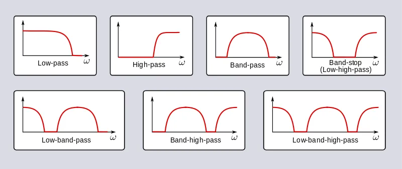
Non-exact design filters have a less severe transition from the passband to the stopband, which is preferable and more suitable in practical situations.
Consequently a transition region is introduced between the two main frequency-bands.
Graphically, such filters give results, that look like this:

[Image 2]
Series R-C Filter Approximation
A simple approximation of a frequency-selective filter is the series RC circuit. The output taken across the capacitor "rejects" high frequencies and can be used as an approximation of a low-pass filter. On the other hand, the output across the resistor "rejects" low frequencies, and as such approximates high-pass filters.
A simple series R-C circuit is of the following form:

[Image 3]
Using Kirchhoff's Laws its possible to define the circuit mathematically as:

Using the Fourier transform results in:

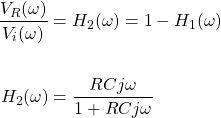
As such, considering the voltage across the capacitor, Vo(ω), the low-pass filter can be described as:

Considering the voltage across the resistor, VR(ω), gives us the high-pass filter:

Moving Average Filter Approximation
In the case of Discrete-Time, moving average filters tend to be used. Such filters have finite-length impulse response and average together adjacent values as they move through them. This procedure is commonly used in the stock market to smooth out the day-to-day fluctuations and in turn to represent long-time trends. In filters, this means retaining lower frequencies and rejecting (smoothing out) high frequencies.
Mathematically, moving average filters looks like this:

Recursive moving average filters are also commonly used for discrete-time filters.
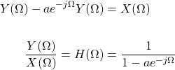
A simple first-order difference equation can easily approximate such a low-pass or high-pass filter:

Using the Fourier transform and its various properties leads us to:

The final result is the Fourier transform of h[n] = an u[n].
RESOURCES:
References
Images
Mathematical equations used in this article were made using quicklatex.
Block diagrams and other visualizations were made using draw.io and GeoGebra
Previous articles of the series
Basics
- Introduction → Signals, Systems
- Signal Basics → Signal Categorization, Basic Signal Types
- Signal Operations with Examples → Amplitude and Time Operations, Examples
- System Classification with Examples → System Classifications and Properties, Examples
- Sinusoidal and Complex Exponential Signals → Sinusoidal and Exponential Signals in Continuous and Discrete Time
LTI Systems and Convolution
- LTI System Response and Convolution → Linear System Interconnection (Cascade, Parallel, Feedback), Delayed Impulses, Convolution Sum and Integral
- LTI Convolution Properties → Commutative, Associative and Distributive Properties of LTI Convolution
- System Representation in Discrete-Time using Difference Equations → Linear Constant-Coefficient Difference Equations, Block Diagram Representation (Direct Form I and II)
- System Representation in Continuous-Time using Differential Equations → Linear Constant-Coefficient Differential Equations, Block Diagram Representation (Direct Form I and II)
- Exercises on LTI System Properties → Superposition, Impulse Response and System Classification Examples
- Exercise on Convolution → Discrete-Time Convolution Example with the help of visualizations
- Exercises on System Representation using Difference Equations → Simple Block Diagram to LCCDE Example, Direct Form I, II and LCCDE Example
- Exercises on System Representation using Differential Equations → Equation to Block Diagram Example, Direct Form I to Equation Example
Fourier Series and Transform
- Continuous-Time Periodic Signals & Fourier Series → Input Decomposition, Fourier Series, Analysis and Synthesis
- Continuous-Time Aperiodic Signals & Fourier Transform → Aperiodic Signals, Envelope Representation, Fourier and Inverse Fourier Transforms, Fourier Transform for Periodic Signals
- Continuous-Time Fourier Transform Properties → Linearity, Time-Shifting (Translation), Conjugate Symmetry, Time and Frequency Scaling, Duality, Differentiation and Integration, Parseval's Relation, Convolution and Multiplication Properties
- Discrete-Time Fourier Series & Transform → Getting into Discrete-Time, Fourier Series and Transform, Synthesis and Analysis Equations
- Discrete-Time Fourier Transform Properties → Differences with Continuous-Time, Periodicity, Linearity, Time and Frequency Shifting, Conjugate Summetry, Differencing and Accumulation, Time Reversal and Expansion, Differentation in Frequency, Convolution and Multiplication, Dualities
- Exercises on Continuous-Time Fourier Series → Fourier Series Coefficients Calculation from Signal Equation, Signal Graph
- Exercises on Continuous-Time Fourier Transform → Fourier Transform from Signal Graph and Equation, Output of LTI System
- Exercises on Discrete-Time Fourier Series and Transform → Fourier Series Coefficient, Fourier Transform Calculation and LTI System Output
Final words | Next up
And this is actually it for today's post!
Next time we will get into Modulation...
See Ya!

Keep on drifting!


