[Image1]
Introduction
Hey it's a me again @drifter1!
Today we continue with my mathematics series about Signals and Systems in order to cover Sampling.
So, without further ado, let's get straight into it!
Sampling Theorem
The sampling theorem is a direct consequence of the modulation theorem and very easy to understand. It basically specifies the minimum sapling rate that has to be used in order to be able to recontruct a continuous-time signal. When uniformly sampled (equally spaced samples) at more than twice the highest frequency present in the signal its possible to recover the original signal. Let's also note that the signal is then uniquely recoverable.
Mathematically, if ωM the highest/max frequency present in the signal (or band limit of the signal), the sampling rate ωS has to be:

Sampling and Reconstruction
Through the sampling theorem its possible to represent band-limited continuous-time signals as a sequence of samples, and so as discrete-time signals. In order to reconstruct the original signal, the impulse train of samples is passed through an ideal low-pass filter.

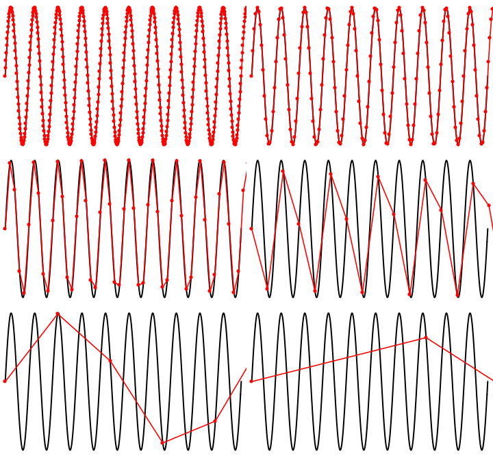
This whole procedure is of course only successful when the relation between the sampling rate and highest frequency is met. As such the reconstructing low-pass filter always generates a reconstruction-consistent signal, even when the sampling condition is violated. But, will reconstruct a signal that is identical to the original signal only when the signal is bandlimited by less than half the sampling frequency, which matches the given set of samples.
For example, the following GIF shows how the sampling frequency affects the sampling of a simple sinusoidal signal:

[Image 2]
Aliasing
When the conditions of the sampling theorem are violated, the frequencies in the original signal which are above half the sampling frequency are reflected down to frequencies below half the sampling frequency. This leads to distortion, which is referred to as aliasing, because higher frequencies take on the alias of lower frequencies.
The concept is far easier to understand in the context of sinusoidal signals. Many continuous-time sinusoids can be taken as samples of a simple sinusoidal signal. If it so happens that all samples have equal height the frequency becomes zero and so there is no clear way of determining which continuous sinusoid was sampled. In this case, the reconstruction filter will make its assumptions for the frequency an reconstruct with constant output. In other words, the sampling frequency will be aliased down to zero frequency (or DC).
In the presence of aliasing an ideal low-pass filter cannot reconstruct the original signal, but samples of the reconstructed signal will always match the samples of the original signal. Sometimes aliasing might also be desirable, specifically when using pulses of light, where aliasing can be used to alias into much lower frequencies that can be seen.
RESOURCES:
References
Images
Mathematical equations used in this article were made using quicklatex.
Block diagrams and other visualizations were made using draw.io and GeoGebra
Previous articles of the series
Basics
- Introduction → Signals, Systems
- Signal Basics → Signal Categorization, Basic Signal Types
- Signal Operations with Examples → Amplitude and Time Operations, Examples
- System Classification with Examples → System Classifications and Properties, Examples
- Sinusoidal and Complex Exponential Signals → Sinusoidal and Exponential Signals in Continuous and Discrete Time
LTI Systems and Convolution
- LTI System Response and Convolution → Linear System Interconnection (Cascade, Parallel, Feedback), Delayed Impulses, Convolution Sum and Integral
- LTI Convolution Properties → Commutative, Associative and Distributive Properties of LTI Convolution
- System Representation in Discrete-Time using Difference Equations → Linear Constant-Coefficient Difference Equations, Block Diagram Representation (Direct Form I and II)
- System Representation in Continuous-Time using Differential Equations → Linear Constant-Coefficient Differential Equations, Block Diagram Representation (Direct Form I and II)
- Exercises on LTI System Properties → Superposition, Impulse Response and System Classification Examples
- Exercise on Convolution → Discrete-Time Convolution Example with the help of visualizations
- Exercises on System Representation using Difference Equations → Simple Block Diagram to LCCDE Example, Direct Form I, II and LCCDE Example
- Exercises on System Representation using Differential Equations → Equation to Block Diagram Example, Direct Form I to Equation Example
Fourier Series and Transform
- Continuous-Time Periodic Signals & Fourier Series → Input Decomposition, Fourier Series, Analysis and Synthesis
- Continuous-Time Aperiodic Signals & Fourier Transform → Aperiodic Signals, Envelope Representation, Fourier and Inverse Fourier Transforms, Fourier Transform for Periodic Signals
- Continuous-Time Fourier Transform Properties → Linearity, Time-Shifting (Translation), Conjugate Symmetry, Time and Frequency Scaling, Duality, Differentiation and Integration, Parseval's Relation, Convolution and Multiplication Properties
- Discrete-Time Fourier Series & Transform → Getting into Discrete-Time, Fourier Series and Transform, Synthesis and Analysis Equations
- Discrete-Time Fourier Transform Properties → Differences with Continuous-Time, Periodicity, Linearity, Time and Frequency Shifting, Conjugate Summetry, Differencing and Accumulation, Time Reversal and Expansion, Differentation in Frequency, Convolution and Multiplication, Dualities
- Exercises on Continuous-Time Fourier Series → Fourier Series Coefficients Calculation from Signal Equation, Signal Graph
- Exercises on Continuous-Time Fourier Transform → Fourier Transform from Signal Graph and Equation, Output of LTI System
- Exercises on Discrete-Time Fourier Series and Transform → Fourier Series Coefficient, Fourier Transform Calculation and LTI System Output
Filtering, Sampling, Modulation, Interpolation
- Filtering → Convolution Property, Ideal Filters, Series R-C Circuit and Moving Average Filter Approximations
- Continuous-Time Modulation → Getting into Modulation, AM and FM, Demodulation
- Discrete-Time Modulation → Applications, Carriers, Modulation/Demodulation, Time-Division Multiplexing
Final words | Next up
And this is actually it for today's post!
Next time we will get into Interpolation...
See Ya!

Keep on drifting!

