The end of the semester three weeks ago, my trip to MIT two weeks ago and a workshop in Lyon earlier this week delayed a bit my regular posting activities, and of course our citizen science project. However, I am pleased to announce today the fourth episode of our research adventure on Hive.
During the last few weeks, we have installed several (open source) high-energy physics packages, and we have simulated 10,000 collisions describing the production of a pair of top-antitop quarks at CERN’s Large Hadron Collider (LHC). We have then reconstructed the simulated collisions in terms of higher-level objects that could be used for a physics analysis.
This week, we investigate further those simulated collisions and will ‘do some physics’. In other words, we will study the properties of what we simulated in the same way as that followed by particle physicists in their everyday life.
Before anything else, here is first a small recap of the previous episodes of our adventure.
- Episode 1 was about to get started and the installation of the MG5aMC software dedicated to particle collider simulations. We got seven reports from the participants (agreste, eniolw, gentleshaid, mengene, metabs, servelle and travelingmercies). @metabs’ report has to be highlighted as it consists of an excellent documentation on how to get started with a virtual machine running on Windows.
- The second episode was dedicted to making use of MG5aMC to generate 10,000 simulated LHC collisions relative to the production of a top-antitop pair at the LHC. We got eight reports from the participants to the project (agreste, eniolw, gentleshaid, isnochys, mengene, metabs, servelle and travelingmercies).
- The third episode focused on the installation of MadAnalysis5, a piece of software allowing us to simulate detector effects, reconstruct the output of the complex simulations into something easier to grasp, and the analysis of the produced events. We got seven contributions (agreste, eniolw, gentleshaid, isnochys, metabs, servelle and travelingmercies).
If you just found out about this citizen science project today and are interested in it, there is still time to embark. It suffices to start with the first three episodes and the current one, taken one by one, and publish your reports on chain (with the #citizenscience tag). They will be reviewed and commented out. Moreover, I am available (both in chain and on the STEMsocial Discord server) to answer any question. Really any!

[Credits: geralt (Pixabay)]
As usual, before moving on with the main material for the exercises of this week, I acknowledge all participants to this project and supporters from our community: @agmoore, @agreste, @aiovo, @alexanderalexis, @amestyj, @darlingtonoperez, @eniolw, @firstborn.pob, @gentleshaid, @isnochys, @ivarbjorn, @linlove, @mengene, @mintrawa, @robotics101, @servelle, @travelingmercies and @yaziris. Please let me know if you want to be added or removed from this list.
The event content - task 1
As explained in details in an earlier blog, any collision (or event) in a high-energy particle collider involves hundreds of final-state particles. This makes its analysis very unpractical. Last week we discussed how to group all final-state particles into a much smaller number of higher-level objects, namely electrons, muons, taus, jets, photons and missing energy (related to the production of invisible particles such as neutrinos or dark matter).
This week we consider the analysis of those ‘reconstructed-level events’. The starting point is the event file that we have produced, and that should be called myevents.lhe.gz. To analyse it, we start the MadAnalysis5 code (that I will call from now on MA5 for short) that we have downloaded last week:
cd madanalysis5
./bin/ma5
Then, when the prompt ma5> is displayed to the screen, we are ready to import the simulated events:
ma5> import ANALYSIS_0/Output/SAF/_defaultset/lheEvents0_0/myevents.lhe.gz as ttbar
ma5> set ttbar.xsection = 505.491
The first line above allows us to import the generated events (myevents.lhe.gz), and to assign to them the label ttbar. The second line tells MA5 that the production cross section associated with this event sample is 505.491 pb.
I recall two important things here. First, the path to the event sample may be different from the above example. We need to provide the exact location of the file myevents.lhe.gz (absolute and relative paths both work). Second, the cross section value that is used corresponds to the production rate computed with MG5aMC a while ago. I hope you can still access it. Otherwise, feel free to use the above value.
In the last exercise of the project’s episode 3, we asked MA5 to generate a histogram displaying the content of the reconstructed events in terms of high-level objects. Let’s redo this once more, but after setting up MA5 so that generated histograms are normalised to the amount of collisions recorded during the full run 2 of the LHC. For this we need to indicate to the code that the luminosity should correspond to 140 fb-1, in particle physics units.
ma5> set main.lumi = 140
ma5> plot NAPID
ma5> submit
ma5> open
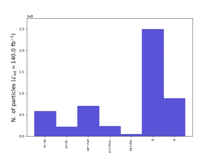
The results should be similar to the image shown below, which is itself very similar to the one generated last time, except for its global normalisation.

[Credits: @lemouth]
This demonstrates that our reconstructed collisions contain a lot of b-jets (the b/b~ column), some electrons (the e+/e- column) and some muons (the mu+/mu- column), very few taus (the ta+/ta- column), some missing energy (the ve/ve~ column), really a lot of jets (the g column) and a bunch of photons (the a column). This is actually a very reasonable finding.
When produced in an LHC collision, a top-antitop pair immediately decays. Each top quark has indeed a lifetime of 10-25 second, so that it can be seen as instantaneously decaying. This decay results in the production of a b-quark and a W boson. A b-quark then gives rise to a jet of strongly-interacting particles in the reconstructed events. As this jet originates from a b quark, we call it a b-jet.
Every single simulated collision should thus produce two b-jets (one from the decay of the top quark and another from the decay of the top antiquark). However, whereas we have the possibility to identify the b-flavour of the jets, this is not a 100%-efficient process. For that reason, we obtain a large amount of b jets (the b/b~ column in the above plot), but in fact not exactly one for each produced top quark or antiquark. Some of the b-jets are then identified as light (i.e. normal) jets (and contribute to the g column in the plot above).
The two W bosons originating from the top-antitop decays also decay instantaneously. This gives rise to either one electron and one neutrino, one muon and one neutrino, a pair of light jets, or a tau lepton and a neutrino. The third of this option is much more frequent than the others, which explains why we see many non-b jets in the event content (the g column in the plot above). Moreover, many extra light jets also come from radiation (see below).
Concerning the W decays into electrons, muons and taus, they should occur with the same rate. However, whereas we can reconstruct with a very good efficiency electrons and muons, this is far from being the case for taus. We expect thus fewer taus compared with the numbers of reconstructed electrons and muons. This is what we see in the figure.
Lepton and photon multiplicity - task 2
It is striking that we have so many light jets and a significant amount of photons in the event final state. The reason is that very energetic particles radiate a lot.
These radiations are often not so energetic. Therefore, we can ‘clean’ the set of interesting objects present in our event’s final states in order to only focus on the objects that have sufficient energy to be issued from heavy stuff (the interesting events are often related to anything that is heavy). Moreover, this also make sure to use reconstructed objects of the best quality. In order to do this in our analysis, we impose that any object that has a ‘transverse momentum’ smaller than 20 GeV is ignored.
Why restricting ourselves on the transverse activity (transverse relative to the beam)? Simply because in the longitudinal direction, we don’t know what is going on. Constituents of the colliding protons are those that actually got annihilated to produce the top-antitop final state of interest. We however have no idea about the energy of these constituents. This ignorance can be bypassed by focusing on the transverse plane. In addition, 20 GeV is reasonable as a threshold for guaranteeing good quality objects in the final state.
Let’s start by considering final-state leptons (electrons, muons and their antiparticles). We implement the restriction (often called a ‘cut’) by typing the following commands in the MA5 command line interface:
ma5> define l = l+ l-
ma5> plot N(l) 5 0 5
ma5> select (l) PT > 20
ma5> plot N(l) 5 0 5
ma5> plot NAPID
ma5> resubmit
ma5> open
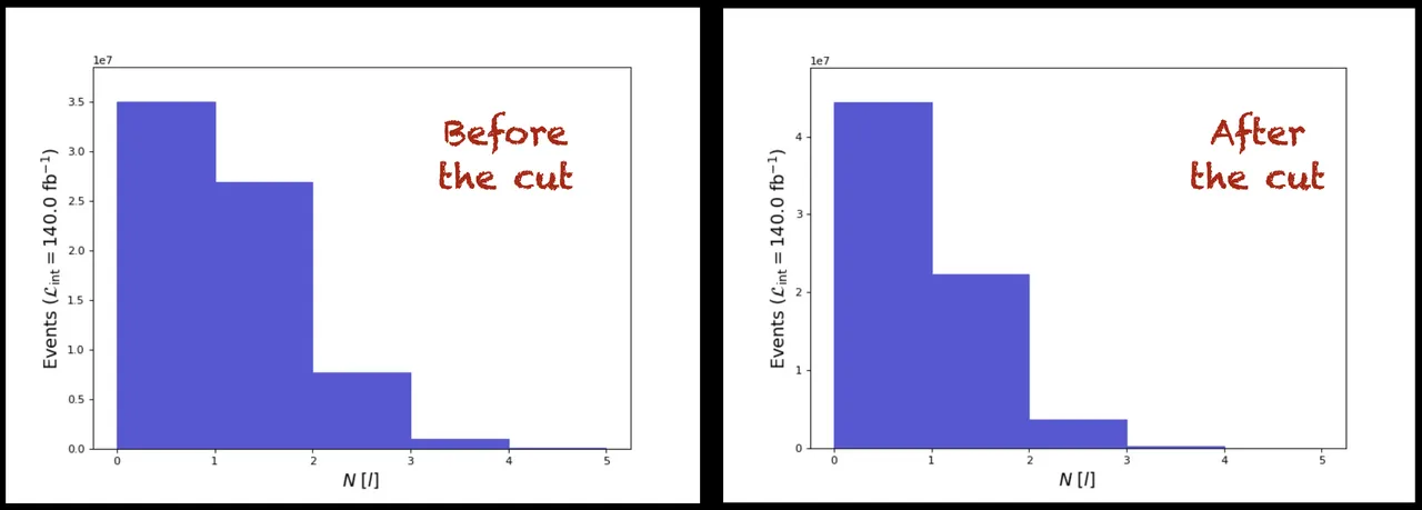
With those commands, we first define a lepton label l that equivalently stands for a muon, an electron, a positron or an antimuon. We then plot the lepton multiplicity in each event. The N symbol indicates that we want the multiplicity in some object, that is provided in parentheses. The last three arguments after the plot command indicate that we want a histogram with five bins (first 5), and ranging from 0 to 5 (last two arguments).
In a second step, we instruct the code to ignore any lepton with a transverse momentum (PT) smaller than 20 GeV (those can be considered as crappy leptons). We finally re-generate the same plot so that we could analyse the impact of the restriction. The results are shown in the image below.

[Credits: @lemouth]
We observe that most events have 0 lepton (the first bin in the left plot), as most of the time the top and antitop quarks decay into particles different from electrons and muons. Then some events have one lepton in the final state (the second bin in the first plot) and a very small number of them have 2 leptons in the final state (the third bin of the first plot).
After the selection (select (l) PT > 20), all leptons that are not so energetic are ignored from the analysis. Each event may hence see its number of leptons decreasing. This is what we observe in the plot: a migration of events from the right part to the left part of the plot.
Let’s now do the same exercise for photons (associated with the label a). We type in the MA5 shell:
ma5> plot N(a) 5 0 5
ma5> select (a) PT > 20
ma5> plot N(a) 5 0 5
ma5> resubmit
ma5> open
At this stage, the meaning of every command can be guessed from the information provided above. If not, feel free to ring the alarm bell in the comment section. The obtained results are given below.

[Credits: @lemouth]
We observe that the selection has the effect of removing most photons (a huge fraction of events ends in the first bin after the selection, which consists of the zero-photon bin). This is consistent with the fact that most photons originate from radiation and are thus not so energetic (or ‘soft’).
Jet multiplicity - homework 1
Knowing that the symbol for a jet is j, I let you investigate how the jet multiplicity varies after a transverse momentum selection of 25 GeV. Note that you may have to vary the bounds of the histogram with respect to what was done in the previous section. Please choose a reasonable upper limit.
Next, you can redo the exercise for b-jets (the symbol being b). Here, you should find very few variations after the selection. Do you have any idea why?
Please post your answers to those questions in your report. Extra rewards will be given to the best ones (and the first ones if identical)!
Selection of a subset of all simulated collisions - task 3
For the moment, we only focused on the multiplicity of the different objects present in the final state of the simulated collisions. We can however study their properties.
To do that, let’s first consider a subset of all generated collisions. For the sake of the example, one of the top quarks will be enforced to decay into one lepton, one neutrino and one b-jet. The other top quark will then be enforced to decay into one b-jet and two light jets.
We thus need to focus on events containing exactly one lepton (and not on any of the other events). Doing so would automatically select the topology introduced above. In practice, this is achieved by typing the following command in the MA5 shell:
ma5> select N(l)==1
As already said, the above selection is called a cut in our jargon. We have a large number of events and we select certain of them satisfying specific properties. We can check the information that is printed in the HTML output of the code. It is shown in the image below.

[Credits: @lemouth]
It indicates that the cut efficiency is of about 30%. This means that about 30% of all events feature exactly one lepton in the final state.
In an ideal signal and background analysis, we need to determine cuts that have a high efficiency for the signal (we keep as much signal as possible) and a small efficiency on the background (we reject as much background as possible). This exercise is often very complicated, especially for hard-to-find rare signals.
Lepton multiplicity after the cut - homework 2
It is now time to play with the code without guidance and study the effect of the above cut on the lepton multiplicity.
What do you expect as a resulting histogram? Is the output in agreement with your expectation?
Lepton properties - task 4
At this stage, we do not know any of the properties of the objects in our event. Among all the standard useful properties of a given object, we have its transverse momentum already introduced (or its energy in some sense), and its pseudo-rapidity that indicates how central an object is in a detector. A small pseudo-rapidity means a very central object and a large one means a very longitudinal one.
Let’s focus on our lepton and study its transverse momentum (PT) and the absolute value of its pseudo-rapidity (ABSETA). To do this, we type in the MA5 interpreter:
ma5> plot PT(l) 25 0 200 [logY]
ma5> plot ABSETA(l) 25 0 2.5 [logY]
ma5> resubmit
ma5> open
Here, we consider two histograms of 25 bins, the transverse momentum distribution ranging from 0 to 200 GeV, and the pseudo-rapidity one from 0 to 2.5. We also indicate the code to use a log scale for the y-axis.
If at this stage the code crashes, please update MA5 from GitHub (I have just fixed a bug due to a change in Matplotlib 18 months ago). A simple git pull from the MA5 installation folder should be sufficient to update the package.
The results should be similar to those in the image below.

[Credits: @lemouth]
This is neither super striking, nor surprising. But those properties are always good to check.
Now let’s move on with something more interesting. In the selected events, one of the produced top quarks decays into a lepton, a neutrino (giving rise to missing transverse energy, MET in the MA5 language) and a b-jet. The other top quark decays into two light jets and a b-jet. Since this proceeds via an intermediate W boson giving rise to the two jets, we should in principle be able to notice this intermediate decay.
In particular, if we mentally combine the two jets, the combined object should be equivalent to a W boson. Therefore, let’s investigate the mass (M) that such a combination of jets would have:
ma5> plot M(j[1] j[2]) 50 0 250 [logY]
ma5> resubmit
ma5> open
In the above command, we decide to focus on the two most energetic of the jets present in the event’s final state. This is why we have j[1] (the most energetic jet) and j[2] (the next to most energetic jet). Then we calculate the mass of the combination and plot it in a histogram that has 50 bins and that ranges from 0 to 250 GeV.
We should get a result similar to that shown below.

[Credits: @lemouth]
We can see here a peak around 80 GeV. This value corresponds to the mass of the W boson. Bingo! This is how we look for the presence of real intermediate particles in a process: we try to reconstruct peaks appearing in the middle of distributions.
Missing transverse energy spectrum - homework 3
As a final question for today, find a way to get the best plot for the missing transverse energy distribution and try to explain where it comes from and if the obtained histogram makes sense. Most information can be found in this post.
As usual extra rewards will be given to the best (and first) results.
Summary: deciphering top pair production at the LHC
I stop here as I think there are already enough things to do and to learn from this blog. Everything that was introduced here will be further used through the course of the project, and this in fact only consists of a kind of appetiser.
I hope you enjoyed the series of exercises proposed today, and feel free to ask for any question or clarification. As usual, please make sure to notify me when writing a report, and to use the #citizenscience tag.
Have a nice week, full of particle physics and I wish everyone good luck for the homework! I will post its solution in 2-3 weeks.