We're already halfway the year 2022 and my schedule for the past weeks have been so crazy. Early this year, I applied for an online course regarding Agent-Based Modeling, which started a few weeks ago (which I'd love to talk about in the future since it requires us to design our own model). I didn't realize that it would run simultaneously with my other commitments. For 2022, I decided to be intentional in learning new skills and exploring different research interests —that's also the reason why I joined Citizen Science on Hive. The learning process has been a mix of short and long strides, but it's great! I have been learning a lot from @lemouth and the progress reports of the other participants.
The set of tasks for this episode of Citizen science is very enjoyable to work on, especially now that particle physicists all over the world are excited as LHC Run 3 started a few weeks ago. And also, one of our tasks involves reproducing a plot from the reference journal of this project.
Just a recap on what we have done so far:
- Installation of the tools [MG5aMC] necessary for particle physics simulation
- Using the MG5aMC to simulate top quark production at CERN's LHC
- Installation and use of MadAnalysis 5 for detector simulation and event reconstruction
- Investigating top quark production at CERN's LHC using MadAnalysis 5
Our current tasks is somewhat a realization that we're nearing to the focus of this project, which tackles the testing of neutrino mass models. A great article about neutrino masses can be read here, surely you can get an understanding of how neutrino masses are investigated beyond the Standard model.
On the second episode of the Citizen Science project, we have used the software MG5aMC for the simulations. And again, it will be our tool for simulating a signal of a new phenomenon. Simulated collisions produced in MG5aMC comprise the signal and the background. Our goal is to to design an appropriate analysis, or a selection strategy, in which various event properties are calculated. Then afterwards, use these calculations to determine whether a given event is kept or rejected. But for this episode, our focus will be on the signal only. So let's begin!
Installing a particle physics model in MG5aMC
To simulate the signal in MG5aMC, we first need to add the model of physics considered in its model database. The UFO model is documented in this scientific paper which I have added to my reading list already. The addition of this model is done by:
cd MG5_aMC_v2_9_9/models

curl https://feynrules.irmp.ucl.ac.be/raw-attachment/wiki/HeavyN/SM_HeavyN_NLO_UFO.tgz > model.tgz

tar xf model.tgz

rm -f model.tgz
This will require you to go to your working directory of MG5aMC. After entering those commands in your terminal, you will be able to see the folder SM_HeavyN_NLO in the models sub-directory of MG5_aMC. Before I proceed, this report would focus on the steps of the simulation tasks of up to the reproducing the plot of the signal rate dependence on the neutrino mass.
Preparing the simulation of a heavy neutrino signal
To start, we start MG5aMC using the command
./bin/mg5_aMC. I have set my terminal to run on Python 3 as default, so I needed to convert the UFO model using the first line of the code block below.MG5_aMC>set auto_convert_model T
MG5_aMC>import model SM_HeavyN_NLO
MG5_aMC>define p = g u c d s u~ c~ d~ s~
MG5_aMC>define j = p
MG5_aMC>generate p p > mu+ mu+ j j QED=4 QCD=0 $$ w+ w- / n2 n3
MG5_aMC>add process p p > mu- mu- j j QED=4 QCD=0 $$ w+ w- / n2 n3
MG5_aMC>output test_signal
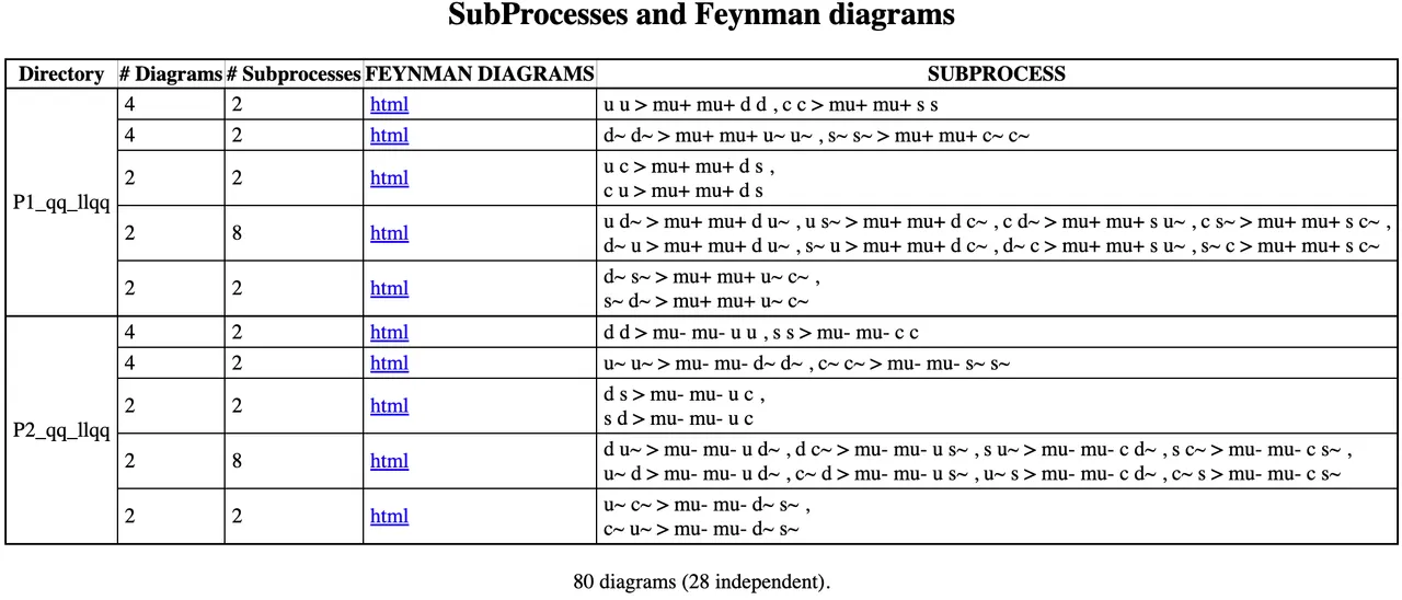
The rest of the code in this block tells MG5aMC of the process we are interested of generating simulations of, which is a proton-proton collision. This results to the Feynman diagrams associated with the process. The different Feynman diagrams show the particle interactions of the sub processes. Each sub processes are unique with its corresponding initial and final state. The different Feynman diagrams which accounts the quarks that make up the protons that collided in the simulation.
Calculating the signal production rate
Following the parameters needed to be changed in the
param_card.dat and run_card.dat
in the reference blog , I was able to obtain a cross section of 0.012 pb. This took around 6-7 minutes using my computer, although the terminal shows around 21 minutes since I had to redo the parameters I have input, I missed one and got an error.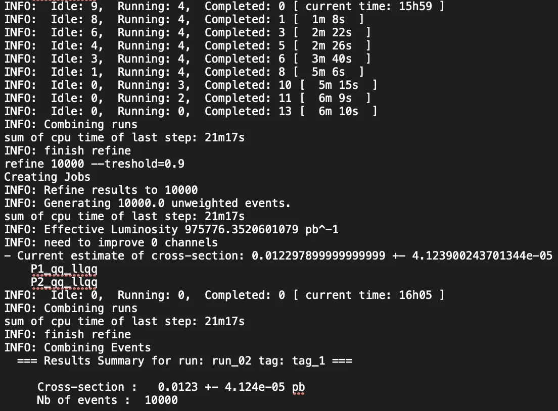
Signal rate dependence on the neutrino mass
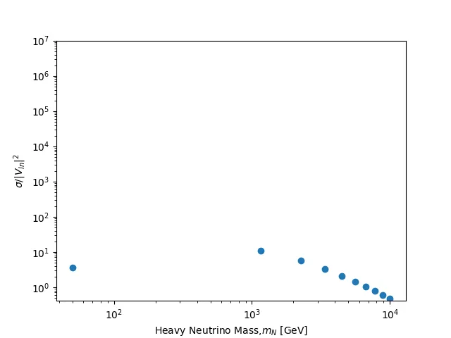
Here's the last part of this progress report, which was exciting for me since for my initial simulation, I have considered 10 points for the mass parameter. This results to 10 runs of the previous task. I had a waiting time of around 47 minutes for this task. The image below shows the result of my scan, the masses I have considered are 10 point interval between the range [50,10000] using numpy linspace:
mass = np.linspace(50,10000,10)
. I did this since my initial goal is to see if I can reproduce the plot.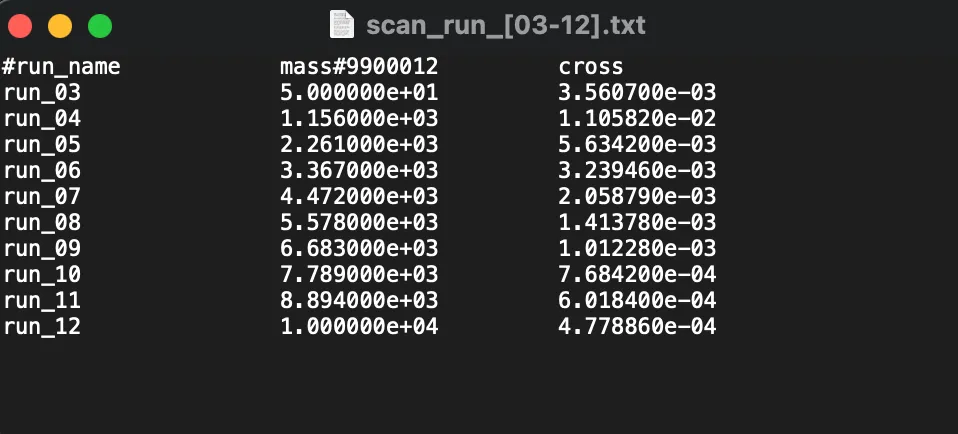
Since I plan to add more data points to achieve a smooth curve and a good representation as well, I have made a Python script to plot the results from this .txt file using matplotlib. I had to make trial and error with setting the delimeter as I try to read this .txt file into a dataframe. Since the unit of the rate in the reference is in fb, I added a multiplier 1000 to the resulting cross section which is in pb.
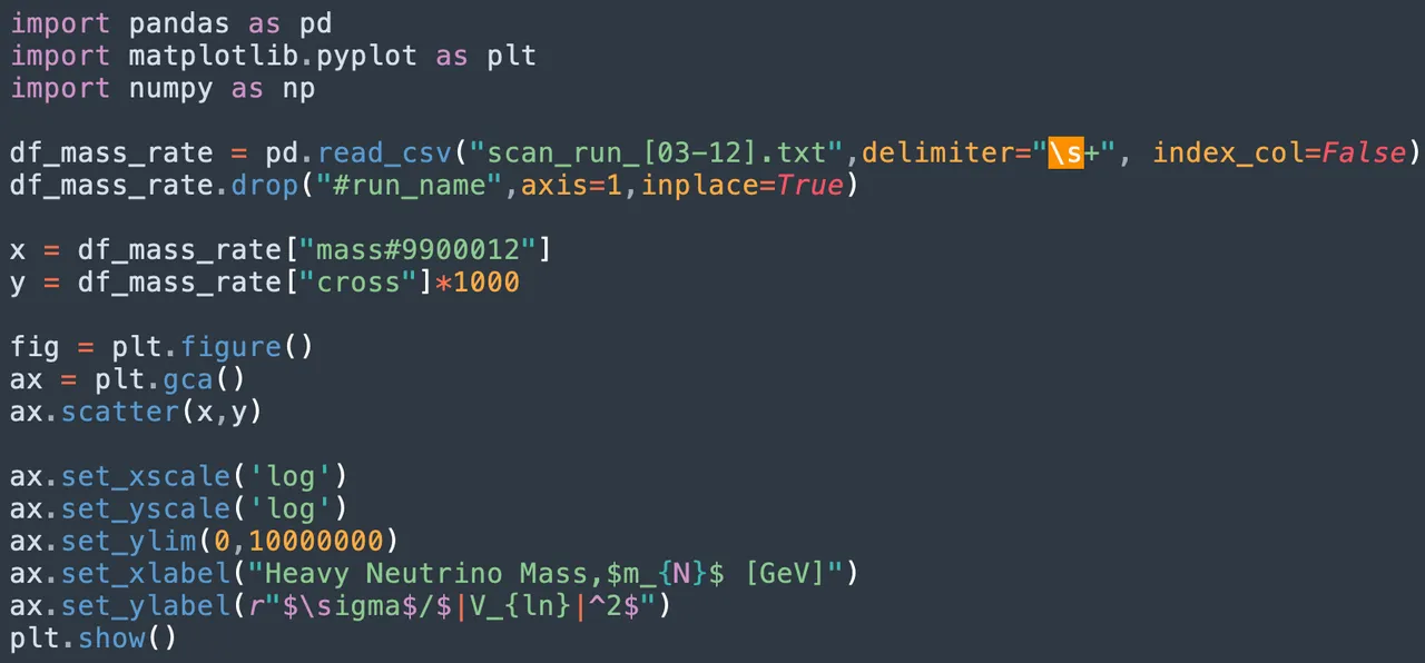
Here's the plot of the results I got, comparing it to the reference paper, I think that the points follow on the curve. I plan to redo this part of the task and consider more mass data points. For now, I used scatter plot since I only considered 10 data points for the masses. The runs I have done only total to 20mb in size, this includes the 10 data points for the masses and the run for calculating the signal production rate.
That's it for now. I'll continue on the simulations of the other tasks when I'd get to sit in front of my computer again after this weekend.