Theoretically, this is my third year of career, I have really enjoyed it, studying at Simon Bolivar University has taught me much more than numbers.

In the virtual classes modality my numerical methods teacher wants us to apply data interpolation from the parameterization of functions with Octave.

What is GNU Octave

Source

Is a free software mainly intended for numerical calculation. It let you solve linear and nonlinear number problems and for performing other number experiments using a language that is compatible with Matlab.

After having applied Octave for some numerical resolution of engineering problems, I was struck by the possibility of processing images in it.
The Octave-forge Image package provides functions to process images, you can do the extraction of characteristics of the same, know the statistics of that, perform spatial and geometric transformations, morphological operations and much more.

Processing Hive's logo in Octave

Source

Today I will process the Hive's logo in Octave in order to reconstruct it from point interpolation using the octave spline function.
In the field of numerical analysis, a spline is a differentiable curve defined in portions by polynomials.
In interpolation problems, splines are often used because they give very accurate results requiring only low-grade polynomials to be used, thus avoiding the undesirable oscillations found when interpolating using high-grade polynomials.

This image is in color, that is to say that each pixel is made up of 3 numbers and each number represents the intensity in one of the basic colors, be it red, blue or green (RGB). Our computer stores the images as a 3-matrix structure, which in this case is 2000/2000 pixels in size; each matrix is called "channel".

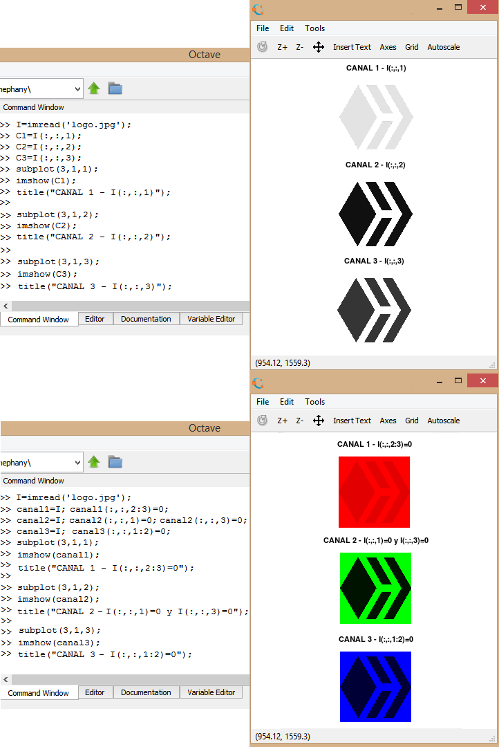
To see that in Octave, we first define a variable "I" as the function >>"imread", in this portion of code, Octave read the image, and "I" is the structure where the three matrices or channels are stored.

Each channel or matrix can present the image by itself, but the image presented by this single channel will be seen on the screen represented in grayscale, that is, colors from 0 (Black) to 255 (White). The figures shown on the right represent each channel, in the first frames you can see that the gray levels in each image are not the same, for example the first channel is lighter than the second and the third channel.

If instead of eliminating the channels, only a value of zero is assigned to the channels that you don't want to present, the result will be the visualization of the image in each channel but using its basics colors (RGB).

The image to process is displayed on the octave canvas with the function >>"imshow". Now, with the >"ginput" function, we define a vector [x, y] with a parameter of 18 since this is the number of points that I am going to capture in the image to be able to do the interpolation.

Thus, this function captures points and returns them as x and y coordinate vectors, once defined it, if you what to see these points use >> "plot (x, y, ’* b’)", where "b" is the abbreviation of the color you want b=blue and "*" to graph points as well as "-" is to graph lines.

As we have for the same value of y, more than one value in x, we must define a new parameter "t" to parameterize the variables X and Y.

Since our logo has peaks (it is not a smooth curve) is not differentiable on this points, so we will apply interpolation for each two points using >>"for" cycles and thus, with a minimum of points we will obtain the desired figure.

Otherwise, we would have something like this:

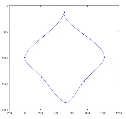
Now x and y depend of t for our splines, so, we create two spline functions >>“pcoef_x1 = spline (t, x1)” and >>“pcoef_y1 = spline (t, y1)”
We define xx1 and yy1 as the “ppval”, which is the function in charge of evaluating the spline and thus project the result of our interpolation with a new plot.

As there are unjoined vertices I create another script with a function called “closedFigure”, whose algorithm is the same as the known one but taking into account the pairs that were left to join.

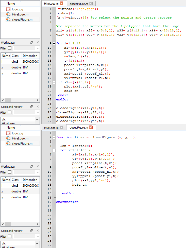
To fill the lines use >>"fill" function and enter the vertices and the desired color, for example to fill the first polygon in red I used >>fill(x11,y11,'r').

Ready! the Hive's logo made in Octave.

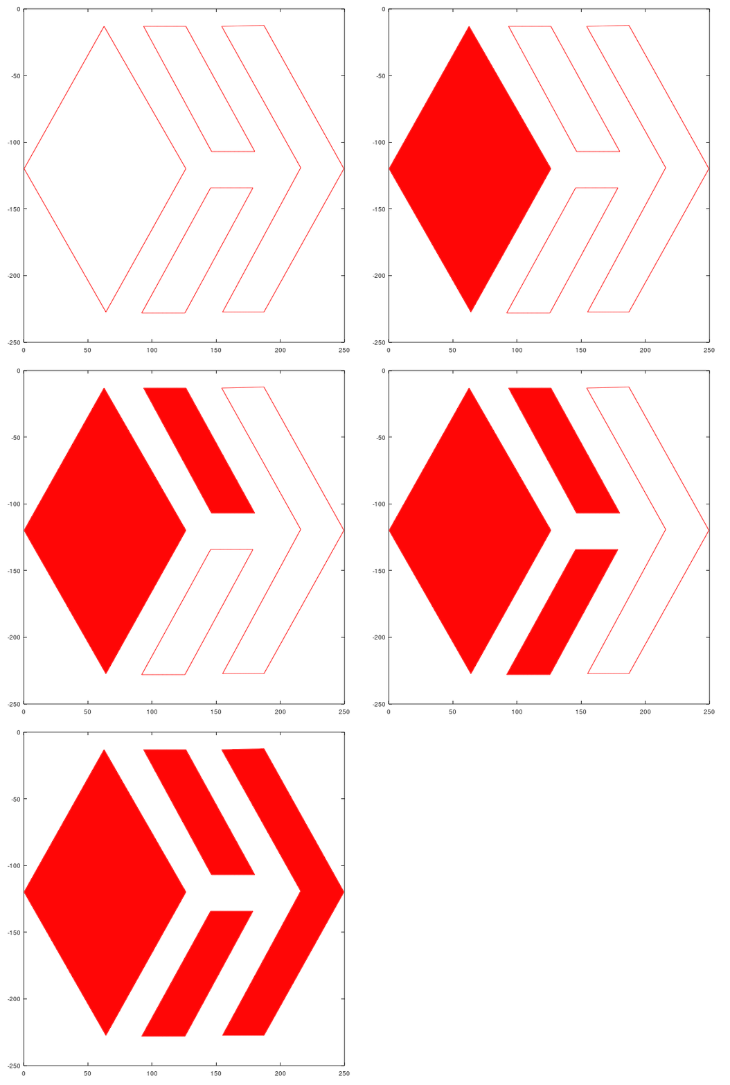
Mission accomplished, I sent the work to my professor (I know it will be something He did not expect), my curious and intelligent colleagues from the university will know in the next few hours our wonderful beehive and now you know a little more about myself and the fascinating uses of Octave.