Citizen Science Entry 5
I'm quickly approaching the last episodes published (so far) in the citizen science series. Next, it's @lemouth's episode 5.
Today, we'll be introducing physics beyond the standard model. Specifically, we'll be augmenting the standard model to include neutrino masses. Most of the details are give in lemouth's episode 5, linked above.
Task 1 - Augmenting the Standard Model
First, we download and install the HeavyN standard model extension:
$ cd ~/physics/MG5_aMC_v2_9_9/models   # Task 1 - Event content
$ curl https://feynrules.irmp.ucl.ac.be/raw-attachment/wiki/HeavyN/SM_HeavyN_NLO_UFO.tgz > model.tgz
$ tar xf model.tgz              # Emits SM_HeavyN_NLO
$ rm model.tgz
$ ls SM_HeavyN_NLO
Task 2 - Heavy neutrino signal
Now it's time to generate more fortran code like we did in earlier episodes. The commands are:
$ cd ~/physics/MG5_aMC_v2_9_9/
$ ./bin/mg5_aMC
MG5_aMC>set auto_convert_model T
MG5_aMC>import model SM_HeavyN_NLO
MG5_aMC>define p = g u c d s u~ c~ d~ s~
MG5_aMC>define j = p
MG5_aMC>generate p p > mu+ mu+ j j QED=4 QCD=0 $$ w+ w- / n2 n3
MG5_aMC>add process p p > mu- mu- j j QED=4 QCD=0 $$ w+ w- / n2 n3
MG5_aMC>output test_signal
I verified that Feynman diagrams were generated and available in ./test_signal/index.html.
As an aside, I had to install ghostscript to ensure Feynman diagrams were generated alongside the HTML. See this MadGraph Q/A.
Assignment 1 - Feynman diagrams
Lemouth poses the question: What are the differences between the Feynman diagrams in the output? And why are there so many diagrams?
What are the differences between diagrams?
Within a row on the output 'info.html' page, it appears Feynman diagrams differ only in the integers attached to the initial and final states. There is no change in the relative positioning of any particles. Also, the Feynman diagrams for each row are associated with one specific subprocess. The other subprocesses included by the row can likely be deduced from the row's generated diagrams. This final point is probably why MadGraph prints 80 diagrams (28 independent) at the bottom of the info page (and generates only 28 diagrams).
Why are there so many Feynman diagrams?
Why are there so many Feynman diagrams? Because there are many ways for the two proton's quarks to interact and produce the processes we specified. For example, two down quarks can interact and produce our desired process. Or two anti-up quarks. Or one down quark and one strange quark.
Task 3
This task requires significant modification to the param_card.dat and run_card.dat files. After executing the output test_signal line shown above, these two files are written to './test_signal/Cards/'. So I modified both files on-disk. I verified that on-disk modification works as opposed to using MadGraph5's prompts.
Here's a diff for the changes I made to param_card.dat and run_card.dat:
--- param_card_default.dat  2022-10-19 18:44:43.032070000 -0700
+++ param_card.dat  2022-10-19 18:51:11.113833000 -0700
@@ -15,9 +15,9 @@
     6 1.733000e+02 # MT
    23 9.118760e+01 # MZ
    25 1.257000e+02 # MH
-  9900012 3.000000e+02 # mN1
-  9900014 5.000000e+02 # mN2
-  9900016 1.000000e+03 # mN3
+  9900012 1.000000e+03 # mN1
+  9900014 1.000000e+09 # mN2
+  9900016 1.000000e+09 # mN3
 ## Dependent parameters, given by model restrictions.
 ## Those values should be edited following the
 ## analytical expression. MG5 ignores those values
@@ -45,15 +45,15 @@
 ## INFORMATION FOR NUMIXING
 ###################################
 Block numixing
-    1 1.000000e+00 # VeN1
+    1 0.000000e+00 # VeN1
     2 0.000000e+00 # VeN2
     3 0.000000e+00 # VeN3
-    4 0.000000e+00 # VmuN1
-    5 1.000000e+00 # VmuN2
+    4 1.000000e+00 # VmuN1
+    5 0.000000e+00 # VmuN2
     6 0.000000e+00 # VmuN3
     7 0.000000e+00 # VtaN1
     8 0.000000e+00 # VtaN2
-    9 1.000000e+00 # VtaN3
+    9 0.000000e+00 # VtaN3

 ###################################
 ## INFORMATION FOR SMINPUTS
@@ -76,7 +76,7 @@
 DECAY  23 2.495200e+00 # WZ
 DECAY  24 2.085000e+00 # WW
 DECAY  25 4.170000e-03 # WH
-DECAY 9900012 3.030000e-01 # WN1
+DECAY 9900012 Auto # WN1
 DECAY 9900014 1.500000e+00 # WN2
 DECAY 9900016 1.230000e+01 # WN3
 ## Dependent parameters, given by model restrictions.
[diff for param_card.dat]
--- run_card_default.dat    2022-10-19 10:40:58.339867000 -0700
+++ run_card.dat    2022-10-19 11:00:23.137437000 -0700
@@ -39,8 +39,8 @@
 #*********************************************************************
 # PDF CHOICE: this automatically fixes also alpha_s and its evol.    *
 #*********************************************************************
-     nn23lo1    = pdlabel     ! PDF set
-     230000    = lhaid     ! if pdlabel=lhapdf, this is the lhapdf number
+     lhapdf    = pdlabel     ! PDF set
+     262000    = lhaid     ! if pdlabel=lhapdf, this is the lhapdf number
 # To see heavy ion options: type "update ion_pdf"
 #*********************************************************************
 # Renormalization and factorization scales                           *
@@ -93,7 +93,7 @@
 # Minimum and maximum pt's (for max, -1 means no cut)                *
 #*********************************************************************
  20.0  = ptj       ! minimum pt for the jets
- 10.0  = ptl       ! minimum pt for the charged leptons
+  0.0  = ptl       ! minimum pt for the charged leptons
  -1.0  = ptjmax    ! maximum pt for the jets
  -1.0  = ptlmax    ! maximum pt for the charged leptons
  {} = pt_min_pdg ! pt cut for other particles (use pdg code). Applied on particle and anti-particle
@@ -182,8 +182,8 @@
 # Store info for systematics studies                                 *
 # WARNING: Do not use for interference type of computation           *
 #*********************************************************************
-   True  = use_syst      ! Enable systematics studies
+   False  = use_syst      ! Enable systematics studies
 #
 systematics = systematics_program ! none, systematics [python], SysCalc [depreceted, C++]
 ['--mur=0.5,1,2', '--muf=0.5,1,2', '--pdf=errorset'] = systematics_arguments ! see: https://cp3.irmp.ucl.ac.be/projects/madgraph/wiki/Systematics#Systematicspythonmodule
-# Syscalc is deprecated but to see the associate options type'update syscalc'
\ No newline at end of file
+# Syscalc is deprecated but to see the associate options type'update syscalc'
[diff for run_card.dat]
Diffs are great for double checking. For reference, the diff for param_card.dat was generated using diff -urN param_card_default.dat param_card.dat.
Now let's launch the simulation by typing launch. Here's the results:
  === Results Summary for run: run_01 tag: tag_1 ===

     Cross-section :   0.0123 +- 4.743e-05 pb
     Nb of events :  10000
Which is inline with lemouth's results.
Assignment 2
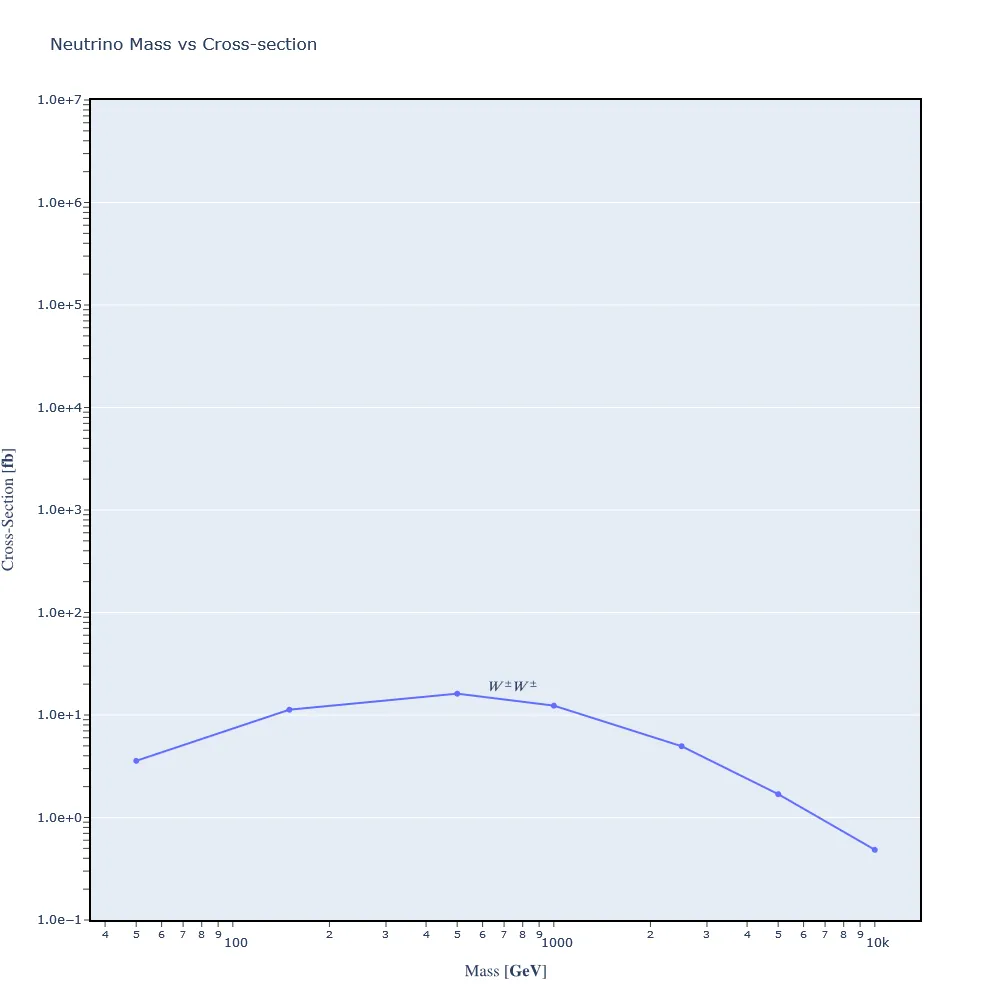
Our job is to reproduce the graph in lemouth's research paper. Per lemouth's advice, I used the 'scan' syntax in param_card.dat to perform the simulation on a finite number of neutrino masses. I scanned through 7: [50,150,500,1000,2500,5000,10000].
Then I launched again using the modified param_card.dat containing the new masses.
When using MadGraph's scan syntax, a 'scan' file is produced with mass and cross-section data. No need to pick through CLI results. Here's the contents of the file:
#run_name            mass#9900012         cross
run_02               5.000000e+01         3.571500e-03
run_03               1.500000e+02         1.126730e-02
run_04               5.000000e+02         1.615130e-02
run_05               1.000000e+03         1.234560e-02
run_06               2.500000e+03         4.962950e-03
run_07               5.000000e+03         1.690980e-03
run_08               1.000000e+04         4.843320e-04
And here's the resulting graph:

This graph is similar to the one found in lemouth's paper. However, there's less fidelity in my version as I sampled only 7 points.
Assignment 3
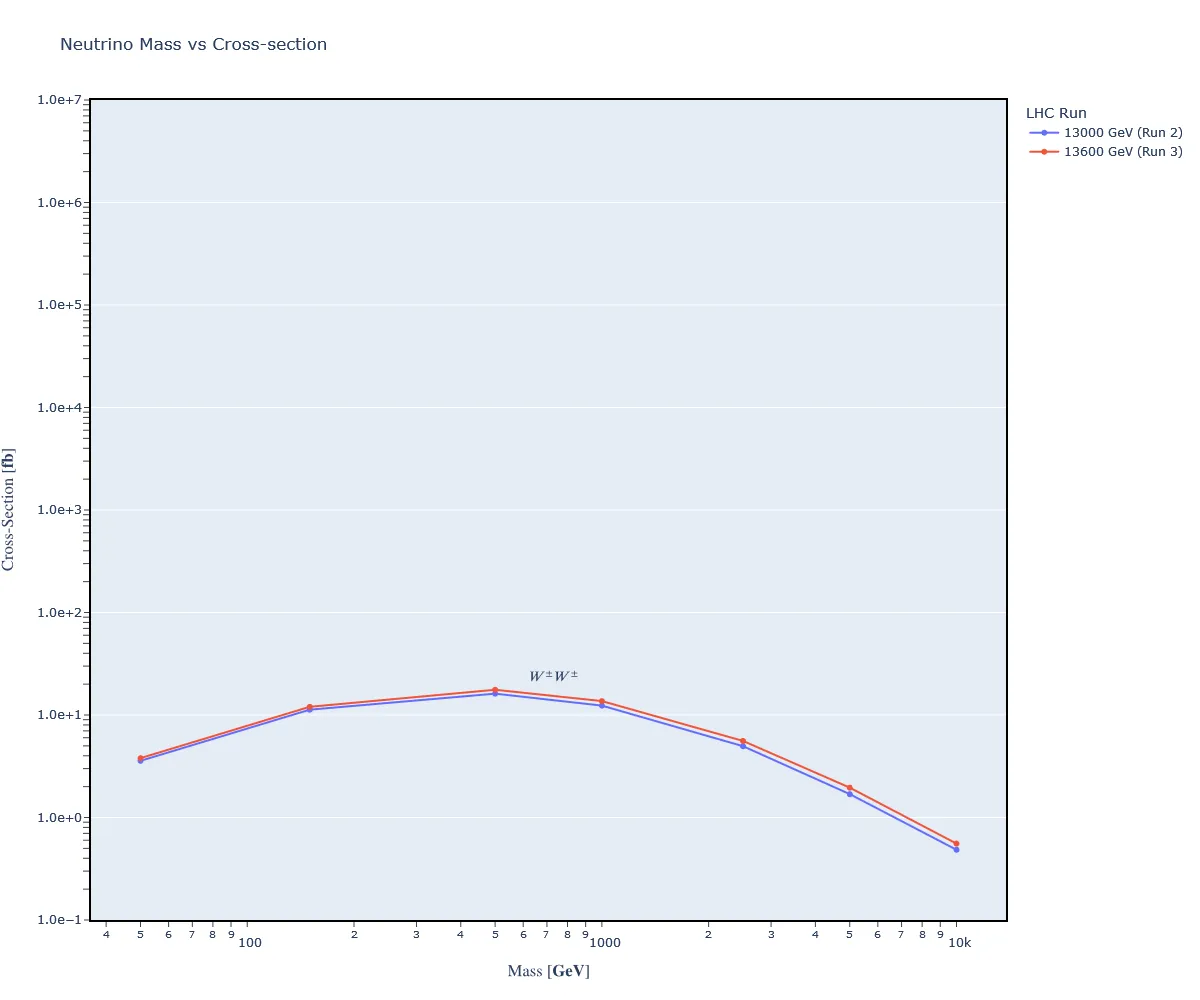
Now we are tasked with rerunning our simulation from Assignment 2. But, this time, we use LHC Run 3 energies. I updated both ebeam1 and ebeam2 in run_card.dat to equal 6800 GeV. Together, they yield a total energy of 13600 GeV.
Here's the data:
#run_name            mass#9900012         cross
run_09               5.000000e+01         3.794100e-03
run_10               1.500000e+02         1.201610e-02
run_11               5.000000e+02         1.762670e-02
run_12               1.000000e+03         1.367100e-02
run_13               2.500000e+03         5.588100e-03
run_14               5.000000e+03         1.955680e-03
run_15               1.000000e+04         5.566650e-04
And the graph:

Here I've overlayed the graph of LHC Run 2 and Run 3.
Conclusion
That's a wrap and another great learning experience. Thanks, lemouth!
I'm looking forward to wrapping up episode 6 before the end of the month. Then, finally, I'll be on the same schedule as everyone else. Yay!
Also, it's great to on-board with such a lovely community. Thanks for having me :).